Tutorials

Main screen

The platform

The CAAos platform was developed in Python 3 language, aiming for a concise, easy to use experience. It is available under GNU GPLv3 license on Github. The installation package and instructions are also available, together with a demo data of two subjects (one healthy control and one stroke patient data), allowing users to operate the platform and its functionalities. Figure 1 presents the home screen of the platform once it is launched.

Figure 1: Platform’s home screen

Menu Entries

There are three main menu entries in the toolbar inside the home screen

(see Figure 2), being them:

1. File: This tab enables the user to exit the platform;

2. Toolboxes: This menu entry allows the user to initiate the patient’s autoregulation analysis by first performing the preprocessing steps, as described in 2.2, and then the cerebral autoregulation analysis;

3. Help: This menu entry contains information about the platform, version, licenses, credits and authors.

   

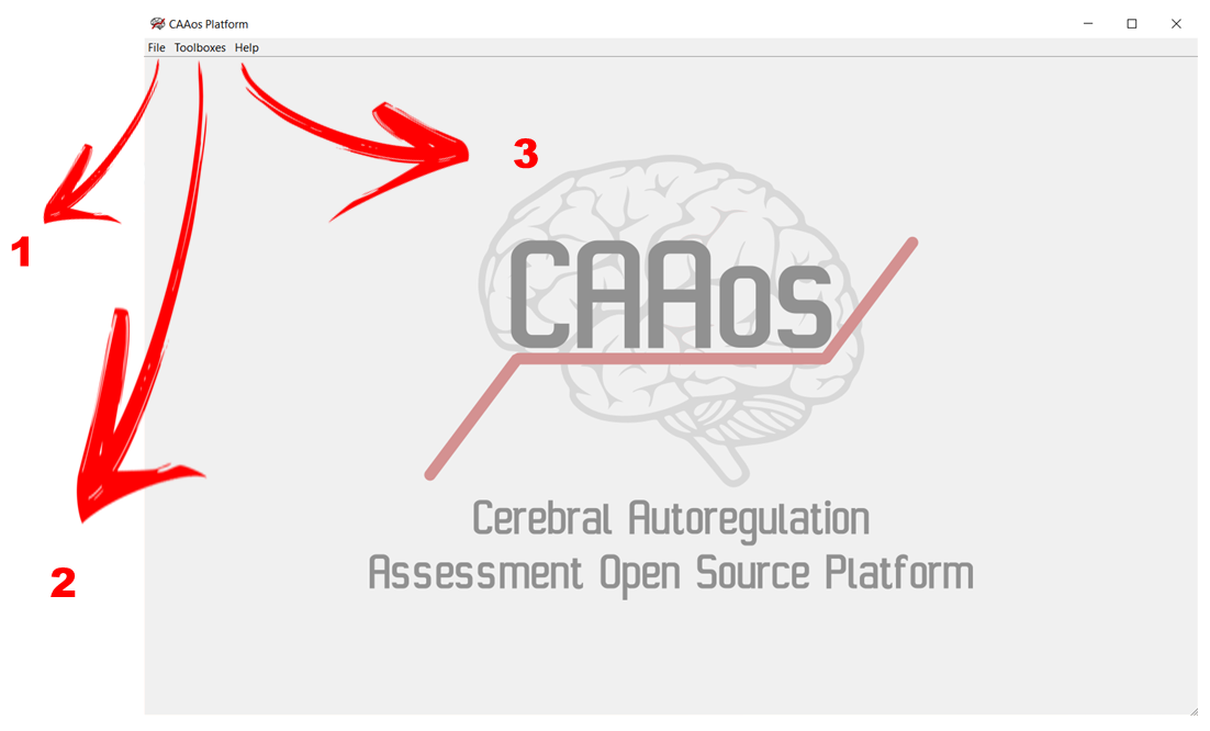
   Figure 2: Indication of the main tabs of the platform.

Usage

Data collection

Before initiating CAAos platform, the user needs to collect the subject’s signals. The signals are the cerebral blood flow velocity (CBFv) and arterial blood pressure (ABP). Other signals such as end-tidal carbon dioxide (EtCO2) can also be uploaded. The first two signals are collected as presented below.

Preprocessing toolbox

Creating and loading a job

Signal analysis starts with the preprocessing toolbox. This toolbox is accessible via Toolboxes menu entry, selecting “Preprocessing”.

The user is then requested to create a new job or load a previously created job file (see Figure 3).

• New job: the platform will request the text file containing the subject’s data.

• Load job: the user is asked to select the job file (.job) previously saved.

  

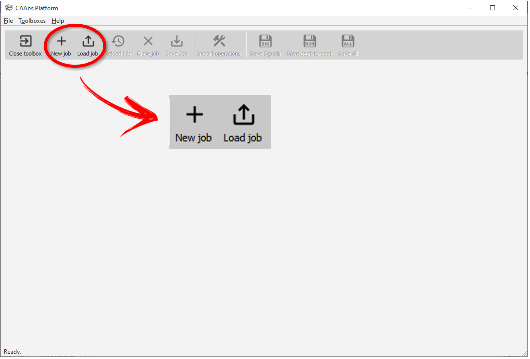
  Figure 3: Creating or Loading a .job file in Preprocessing toolbox.

The platform will load and show the data, as demonstrated in Figure 4.

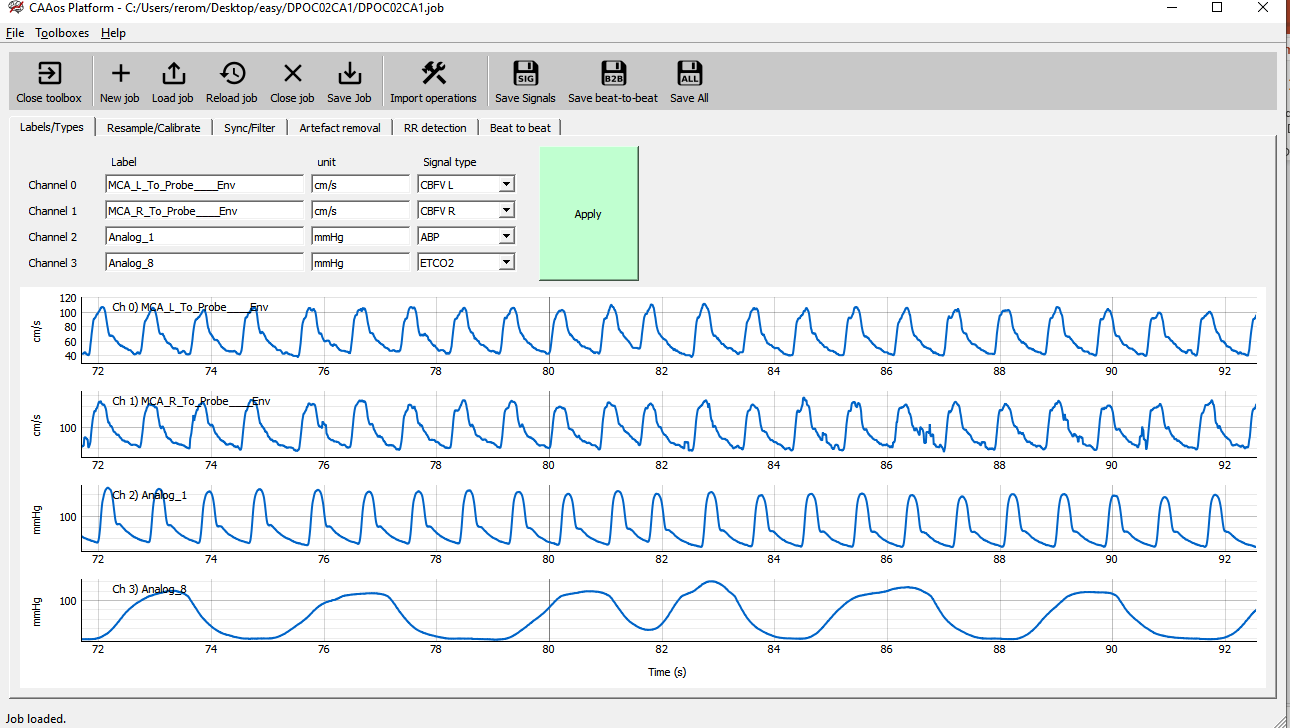
Figure 4: Illustration of the first tab of the platform: Labels/Types.

At this point, the user can start the data preprocessing, which contains the following tabs

• Labels/types

• Resample/Calibrate

• Sync/Filter

• Artefact Removal

• RR detection

• Beat to beat

Labels/Types

When the Preprocessing toolbox opens, it will automatically show the Labels/Types tab, as represented in Figure 4 and Figure 5. On the column “Labels” (Figure 5), the user will see the provisory name of the channels read automatically from the input data heading. In this stage, the user can label the signals following his/her preference. It is presented below an example of labeling the signals.

• Channel 0: Middle Cerebral Artery of the left cerebral hemisphere (Label: CBFv_Left)

• Channel 1: Middle Cerebral Artery of the right cerebral hemisphere (Label: CBFv_Right)

• Channel 2: Arterial Blood Pressure (Label: ABP)

• Channel 3: End-Tidal Carbon Dioxide (Label: ETCO2)

After labeling the signals, the user can select the signals’ unit and then the “Signal Type”. The last columns, Signal Type, is a preconfigured named list, to allow the CAAos platform identify the signals to the cerebral autoregulation analysis.

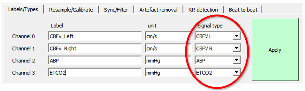
Figure 5: Example of indication of the column signal type.

Observation: Changing the unit will not change the numeric values. This is just a label used to show the results. For changing the unit, please see Resample/Calibrate tab.

The changes will be recorded when the user click on “Apply” button. The plots will be updated when the user click ‘Apply’ (Figure 6). To improve signal visualization, the user can zoom in and zoom out the graphics by using the mouse’s cursor.

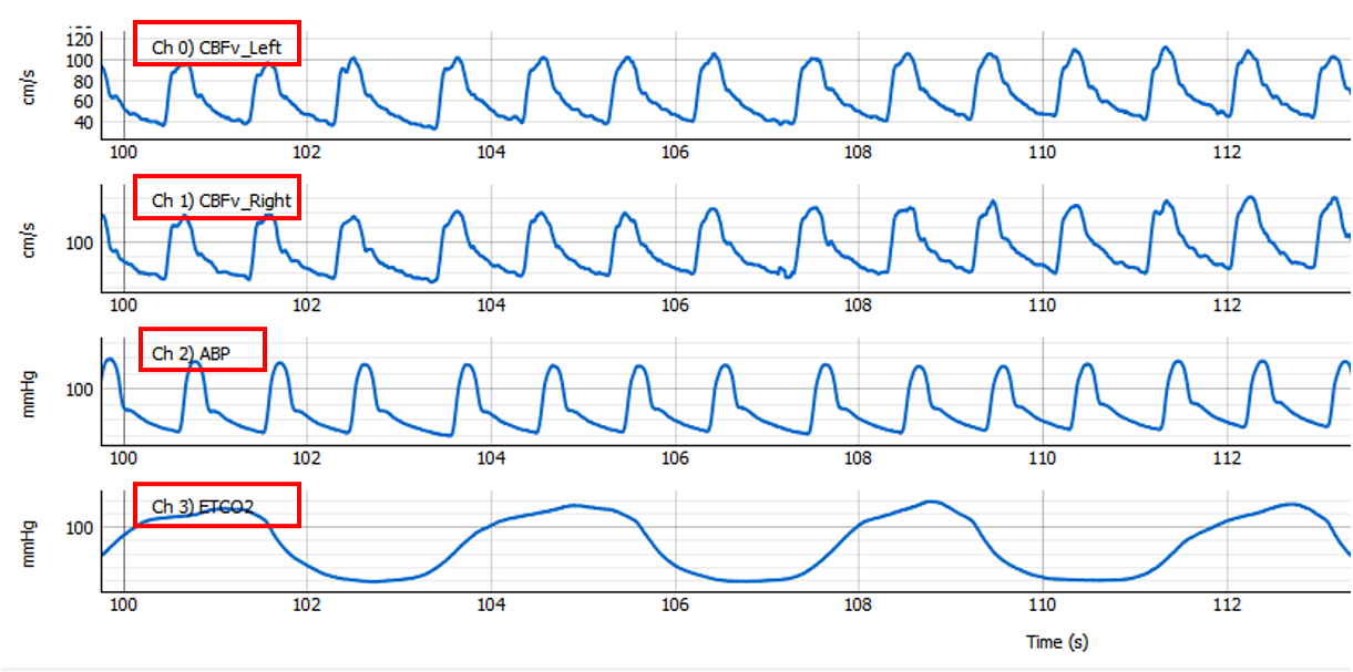
Figure 6: Graphics of the labeled signals.

Resample/Calibrate

Once the settings of Labels/Types is performed, the user can move to the next tab “Resample/Calibrate”, as presented in the Figure 7. In this tab, the user will be able to configure the following settings:

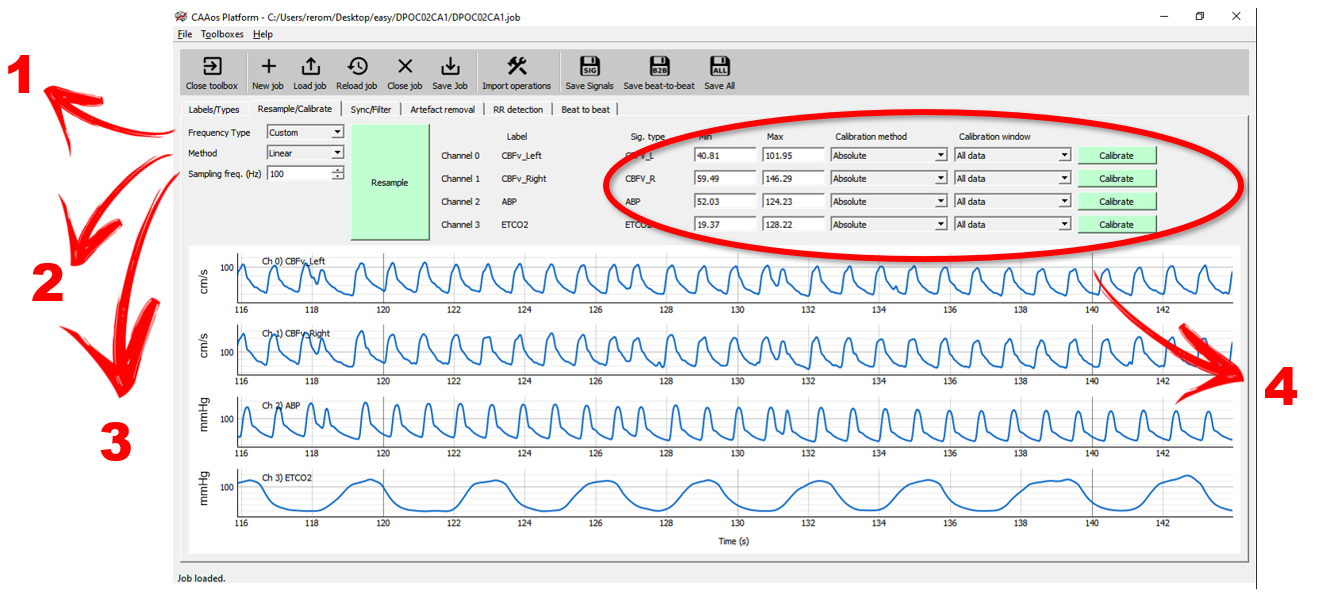
Figure 7: Illustration of the tab Resample/Calibrate with indication of the tools.

1. Sampling Frequency Type: the user may choose among Minimum, Maximum or Customized sampling frequency. Since ABP and CBFv are recorded from different equipments, the sampling frequency can be different between them. See further details below in the “Background” subsection”;

2. Resampling interpolation method: the available methods of interpolation are Zero, Linear, Quadratic or Cubic;

3. Sampling frequency: the CARNet [1] also suggests that sampling frequency of 100 Hz, then user can select “custom” and then define the sampling frequency value;

When this procedure is done, the user can click on “Resample”.

4. Signal calibration: the user may calibrate the signals individually, in special the ABP signal (if the user also measured ABP with another equipment simultaneously, such a sphygmomanometer, prior the beat-to-beat ABP recording). To calibrate a signal, the user need to inform minimum and maximum values. Calibration methods include “Absolute” and “5/95 percentile” and it can be applied to a signal window or to the entire signal data. The user must click on “Calibrate” to finalize the procedure.

Sync/Filter

This tab (Figure 8) provides tools for synchronization and filtration the signals. Synchronization allows performing the synchronization between all signals, since they are acquired using different devices and delays might be present. Filtering is used to remove high frequency noise.

• Highlight 1: the user can select what settings will be applied to each channel, synchronization and/or filtering.

• Highlight 2: apply synchronization to the selected channels.

• Highlight 3: apply the digital filter to the selected channels.

• Sync Methods: select the method between “Correlation” or “Fixed ABP delay”. The second option is the most applied.

• ABP delay: Time delay between ABP and other signals. The timing placed here depends on the equipment that is used to do the ABP reading.

• Filter Type: select the type among “Moving Average”, “Median” and “Butterworth”.

  

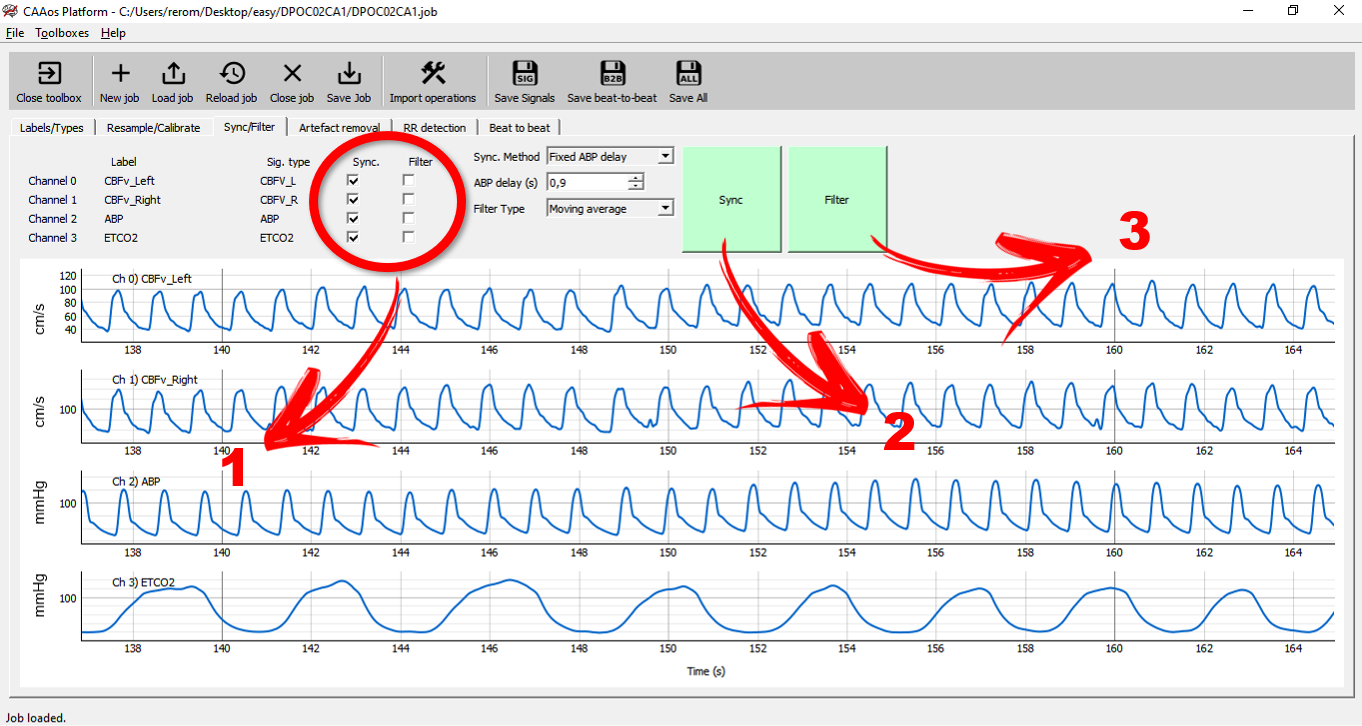
  Figure 8: Illustration of tab Sync/Filter.

Artefact Removal

All signals can be visually inspected to identify artefacts and noise. These can be removed following these general steps (Figure 9):

1. The user visually inspects all the recorded data and identity the artefact. Here the user can zomm in/out with the mouse wheel and pan to the sides by left-clicking and holding while moving to the sides. (Highlight 1 in Figure 9)

2. The user chooses Region Type and Method and click on New selection button to select the area to be excluded (Highlight 2 in Figure 9). A window highlight will appear over the signals.

3. The user can adjust the window size to cover the region of the artefact by moving the window limits to the desired positions.

4. The user click on Remove to clear the artefact.

   

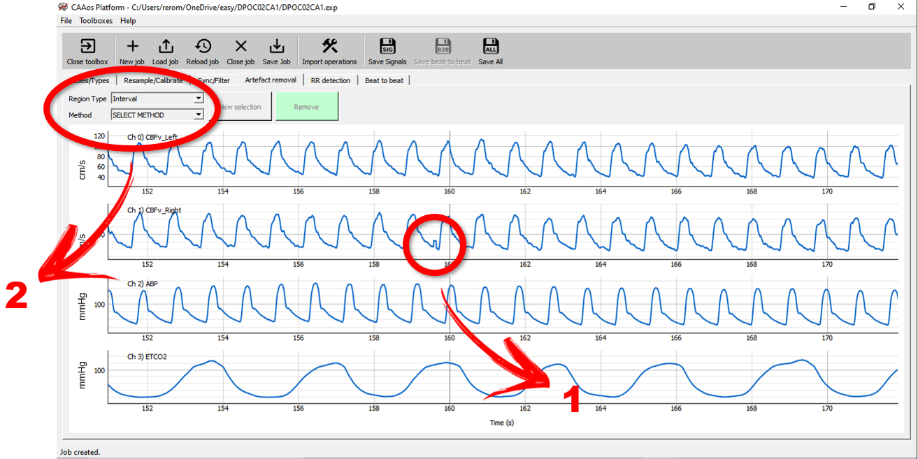
   Figure 9: Illustration of Artefact Removal tab.

Note

Caution: Removing large ranges of the signals can compromise the autoregulation analysis.

Three methods can be used to remove signal artefacts.

• Interpolation: Signals contained in the selected window is replaced by a linear segment connecting the ends. It is indicated to remove small artefacts.

  

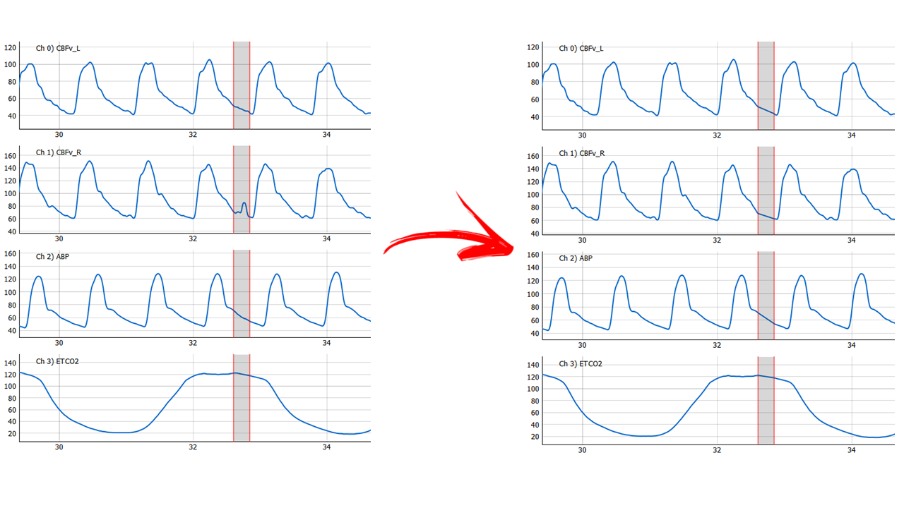
  Figure 10: Interpolation method.

• Crop: This method deletes the selection.

  

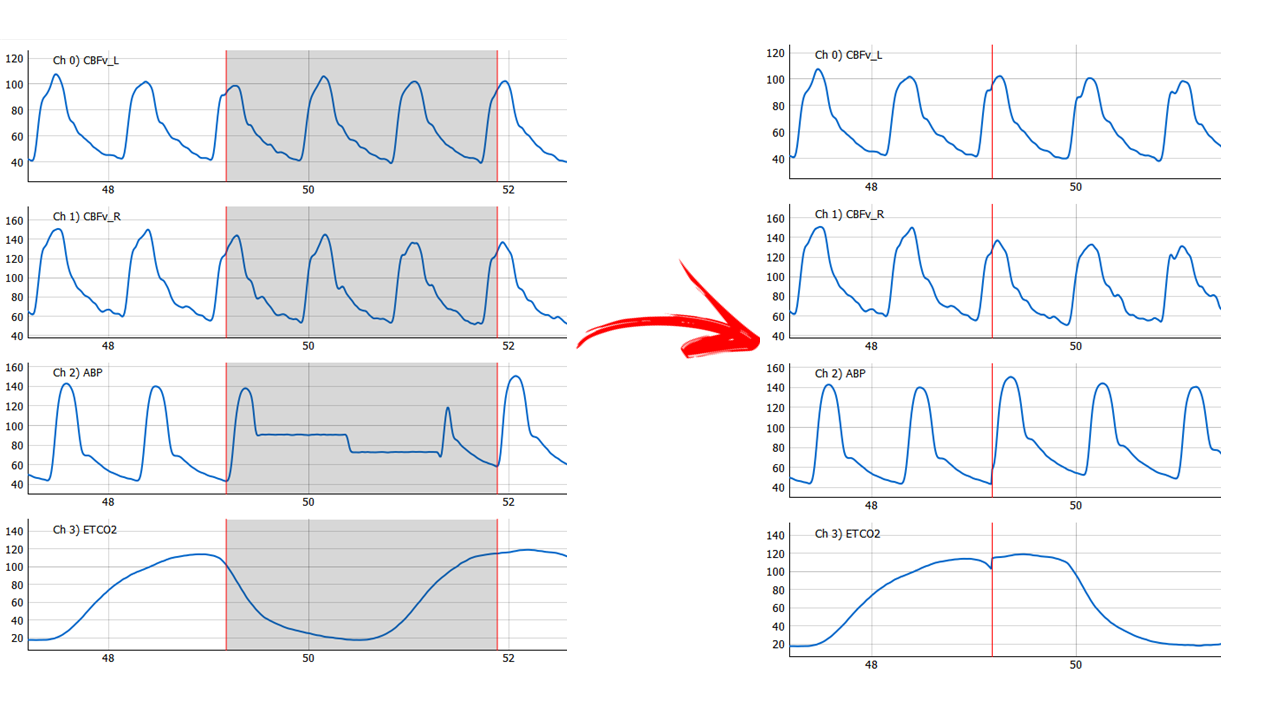
  Figure 11: Crop method.

• Join Peaks: This method is similar to crop method. However the selection is extended to complete a cardiac cycle. It is indicated to remove larger artefacts.

  

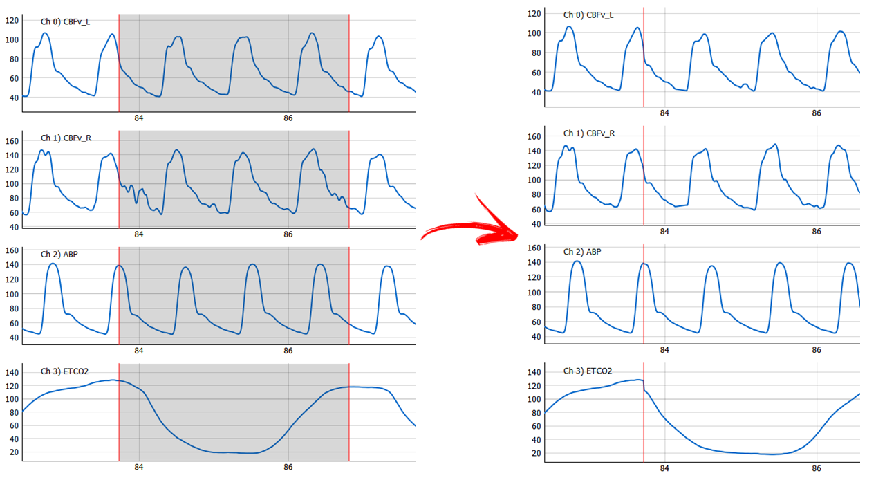
  Figure 12: Join Peaks method. Note that the selection window is extended to the right to enclose a complete signal.

R-R peak detection

The platform finds the systolic peaks from the ABP signal. The detection employs the automatic multiscale-based peak detection (AMPD). Once the user clicks the button Find RR Marks, The peaks are presented as red dots (Figure 13).

The user can add or remove any marks with Add Mark and Remove Mark buttons. The plot on the top right show the heart rate of the patient and can be used to identify missing or extra R-R marks.

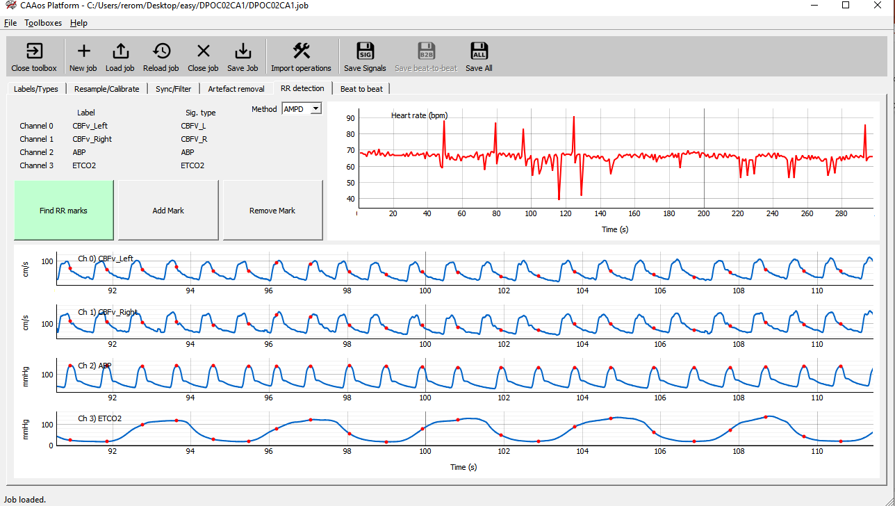
Figure 13: Illustration of RR detection tab.

Beat-to-beat surrogate signal

The last tab of the preprocessing module generates the surrogate beat-to-beat from the loaded signals. To generate the beat-to-beat signals, an upsampling is needed for equidistant sampling intervals and to preserve the relevant frequency range components of cerebral autoregulation.

CARNet[1] suggests spline (third-order piecewise polinomials) interpolation with minimum re-sampling frequency of 4 Hz. After the settings, user needs press the button Extract beat-to-beat and the platform will present the beat-to-beat signals (Figure 13). The user also needs to press the button “Filter” to visualize the signals filtered.

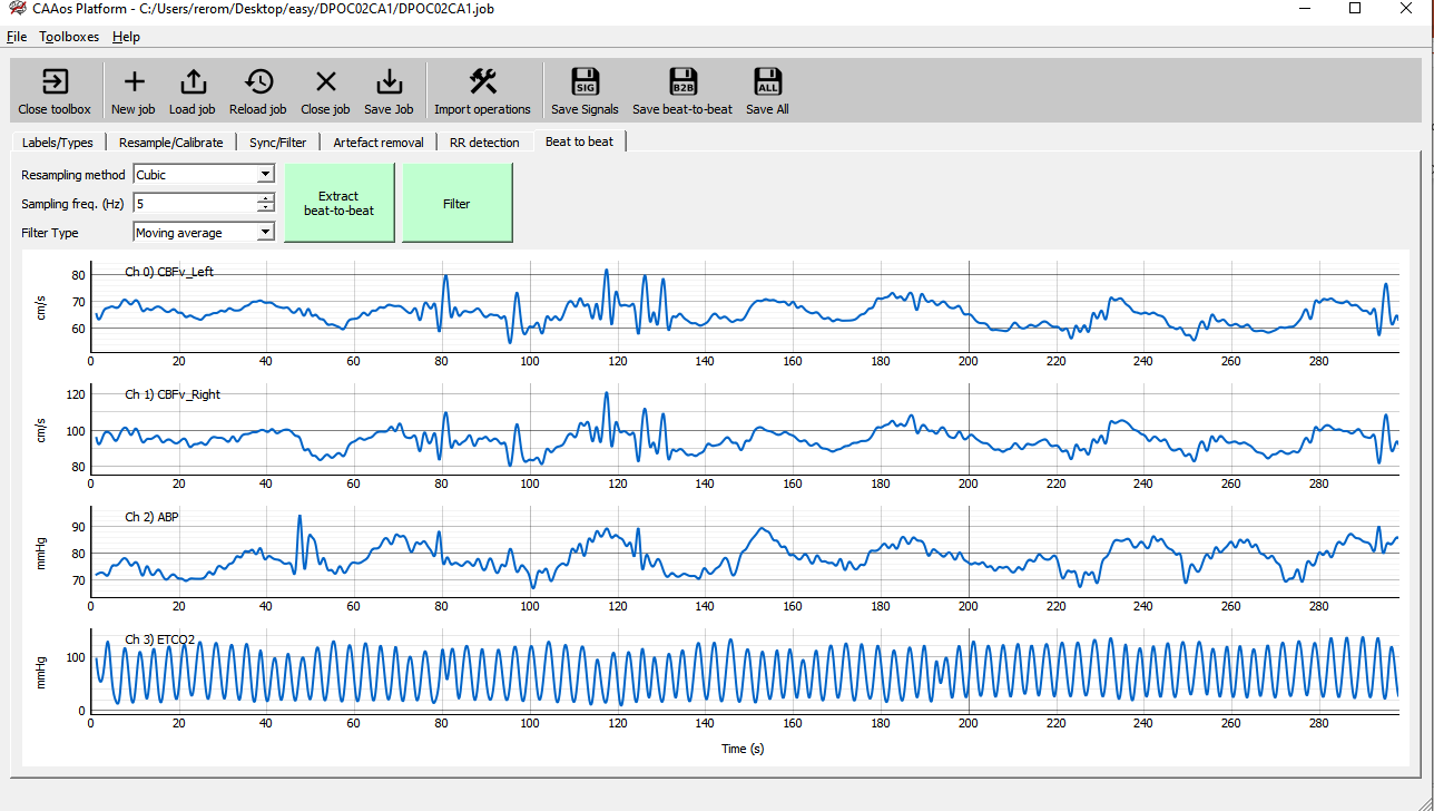
Figure 14: Illustration of beat-to-beat tab.

Saving data

At any point the user can save the job file and/or the processed signals using Save Job, Save Signals buttons on top. If beat-to-beat data is also created, the user can also save them via Save beat-to-beat.